A first DarSIA image

The five-minute tour: read a photograph as a physical Image, inspect it, overlay a metric grid, and cut out a region of interest – either in physical coordinates (metres) or by raw pixel index.

import os

import darsia

IMAGES = os.path.join("..", "images")

Read an image and attach physical dimensions. width and height are the real-world extent of the photograph in metres.

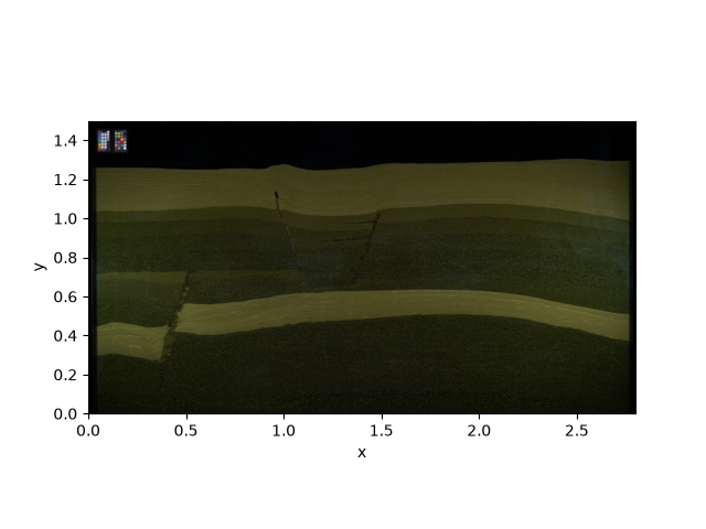
image = darsia.imread(os.path.join(IMAGES, "baseline.jpg"), width=2.8, height=1.5)
image.show("baseline")

Warning: No exif metafile found. Please install ImageMagick to read metadata from terminal.

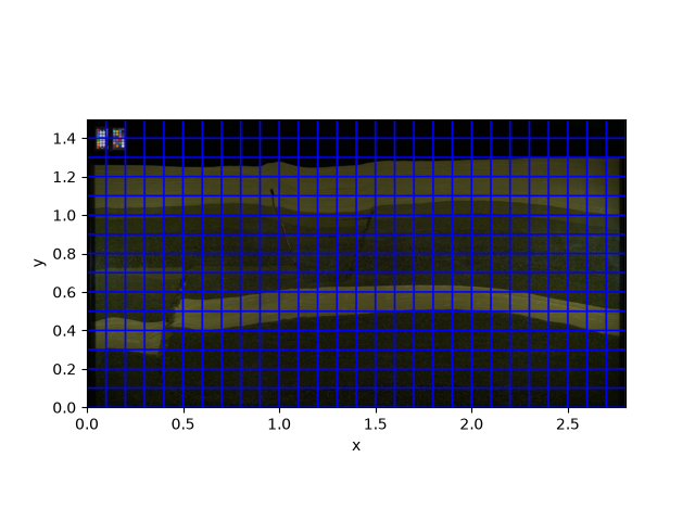
A copy with a 10 cm metric grid drawn on top.

grid_image = image.add_grid(dx=0.1, dy=0.1)
grid_image.show("with grid")

Clipping input data to the valid range for imshow with RGB data ([0..1] for floats or [0..255] for integers). Got range [0.0..125.0].

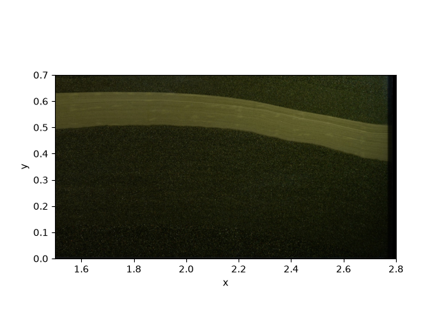
Extract a region of interest given by two physical corner points.

roi = darsia.make_coordinate([[1.5, 0], [2.8, 0.7]])
roi_image = image.subregion(roi)
roi_image.show("region of interest (metres)")

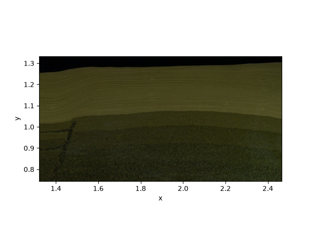
The same call also accepts a tuple of slices to cut a region by raw pixel index – handy when you are reading coordinates straight off the axes.

pixel_roi = image.subregion((slice(200, 900), slice(1500, 2800)))
pixel_roi.show("region of interest (pixels)")

The physical metadata and the raw array are both accessible.

print("metadata:", image.metadata())
print("array shape:", image.img.shape)

metadata: {'space_dim': 2, 'indexing': 'ij', 'dimensions': [1.5, 2.8], 'origin': Coordinate([ 0. ,  1.5]), 'series': False, 'scalar': False, 'date': None, 'reference_date': None, 'time': None, 'name': None, 'type': <class 'darsia.image.image.OpticalImage'>, 'color_space': 'RGB'}
array shape: (1788, 3180, 3)