Earth Mover’s / Wasserstein distance

The distance between two equal-mass distributions, computed with the OpenCV Earth Mover’s Distance and with DarSIA’s Beckmann–Newton solver. The Newton solver also returns the optimal transport fields.

import matplotlib.pyplot as plt
import numpy as np

import darsia

Two blobs of identical total mass at opposite corners of the domain.

mass1_array = np.zeros((80, 140), dtype=float)
mass2_array = np.zeros((80, 140), dtype=float)
mass1_array[20:30, 20:30] = 1
mass2_array[60:80, 120:140] = 1
mass1_array /= np.sum(mass1_array)
mass2_array *= np.sum(mass1_array) / np.sum(mass2_array)

mass1 = darsia.Image(mass1_array, width=70, height=40, scalar=True, dim=2, series=False)
mass2 = darsia.Image(mass2_array, width=70, height=40, scalar=True, dim=2, series=False)

fig, axes = plt.subplots(1, 2, figsize=(9, 3))
axes[0].imshow(mass1.img)
axes[0].set_title("mass 1")
axes[1].imshow(mass2.img)
axes[1].set_title("mass 2")
for ax in axes:
    ax.set_axis_off()
fig.tight_layout()

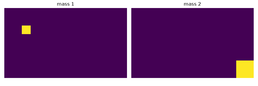
OpenCV Earth Mover’s Distance.

distance_cv2 = darsia.wasserstein_distance(mass1, mass2, method="cv2.emd")
print(f"cv2.emd distance: {distance_cv2:.4f} m")

cv2.emd distance: 14.2842 m

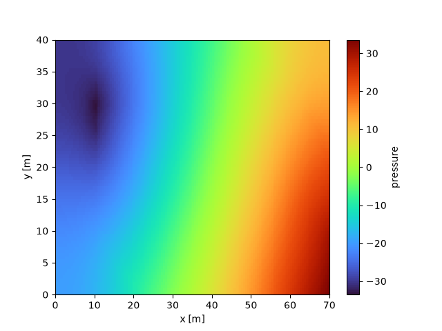
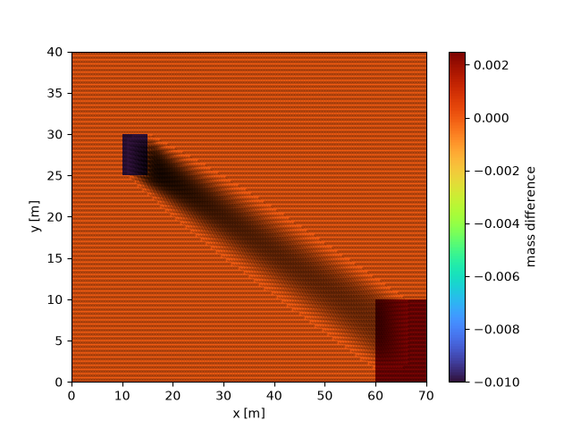
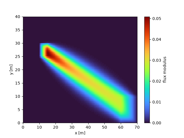
DarSIA Beckmann–Newton solver. Passing return_info yields the optimal flux, pressure and transport density alongside the distance.

options = {
    "num_iter": 100,
    "tol_residual": 1e-10,
    "tol_increment": 1e-6,
    "tol_distance": 1e-8,
    "linear_solver": "direct",
    "verbose": False,
    "return_info": True,
    "formulation": "flux_reduced",
}
distance_newton, info = darsia.wasserstein_distance(
    mass1, mass2, method="newton", options=options
)
print(f"Newton distance: {distance_newton:.4f} m")

/home/runner/work/DarSIA/DarSIA/src/darsia/measure/beckmann_problem.py:1024: RuntimeWarning: divide by zero encountered in divide
  J_inv = sps.diags(self.flux_view(1.0 / jacobian.diagonal()))
Newton distance: 14.3005 m

The transport fields for this solution.

darsia.plotting.plot_2d_wasserstein_distance(
    info, **{"resolution": 1, "save": False, "name": "blobs"}
)
plt.show()

• 
• 
•