Wasserstein: splitting a square

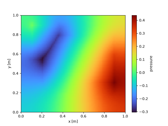
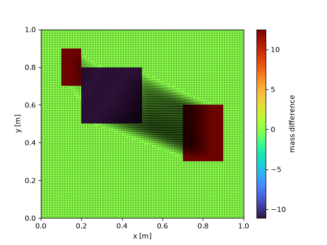
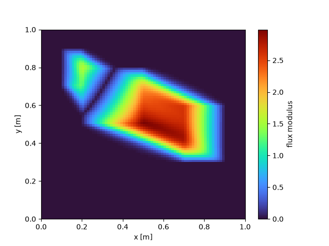
Move a single square of mass onto two target squares of half the mass each, and inspect the optimal flux, pressure and transport density returned by the Beckmann-Newton solver.

import matplotlib.pyplot as plt
import numpy as np

import darsia

Coarse source and target, then normalise to equal integrated mass and refine.

rows = cols = 10
meta = {"width": 1, "height": 1, "space_dim": 2, "scalar": True}

src_square = np.zeros((rows, cols), dtype=float)
src_square[2:5, 2:5] = 1
src_image = darsia.Image(src_square, **meta)

dst_squares = np.zeros((rows, cols), dtype=float)
dst_squares[1:3, 1:2] = 1
dst_squares[4:7, 7:9] = 1
dst_image = darsia.Image(dst_squares, **meta)

geometry = darsia.Geometry(**src_image.shape_metadata())
src_image.img /= geometry.integrate(src_image)
dst_image.img /= geometry.integrate(dst_image)

lvl = 3
resize = darsia.Resize(
    **{
        "resize shape": (rows * 2**lvl, cols * 2**lvl),
        "resize interpolation": "inter_nearest",
    }
)
src_image = resize(src_image)
dst_image = resize(dst_image)

Solve with the Newton solver and a direct linear solver.

options = {
    "num_iter": 100,
    "tol_residual": 1e-10,
    "tol_increment": 1e-6,
    "tol_distance": 1e-10,
    "bregman_update": lambda it: it in [0, 20],
    "linear_solver": "direct",
    "linear_solver_options": {"tol": 1e-6},
    "verbose": False,
    "return_info": True,
    "formulation": "flux_reduced",
}
distance, info = darsia.wasserstein_distance(
    src_image, dst_image, method="newton", options=options
)
print(f"Wasserstein distance: {distance:.4f}")

/home/runner/work/DarSIA/DarSIA/src/darsia/measure/beckmann_problem.py:1024: RuntimeWarning: divide by zero encountered in divide
  J_inv = sps.diags(self.flux_view(1.0 / jacobian.diagonal()))
Wasserstein distance: 0.3770

DarSIA’s built-in visualisation of the solution fields.

darsia.plotting.plot_2d_wasserstein_distance(
    info, **{"resolution": 1, "save": False, "name": "squares"}
)
plt.show()

• 
• 
•